TL;DR
- Lossy compression reduces file size by approximating the original data rather than preserving it exactly, enabling much higher compression ratios compared to lossless methods
- It’s essential for modern content distribution, significantly reducing storage and delivery costs while minimizing buffering and load times
- Lossy techniques balance compression ratio versus distortion: higher compression usually introduces more visible/audio artifacts
- Quality and performance are evaluated using distortion metrics such as Perceptual Distortion, Mean Square Error, and PSNR to quantify how close the compressed output is to the original
- Typical lossy compression involves two steps: 1) Quantization and 2) Transform Coding (e.g., DCT, wavelet-based transforms) that reduce redundancy by representing data in ways easier to compress
This is a comprehensive and detailed guide to Lossy Compression algorithms.
Here you will find everything a developer needs to know about this cutting-edge topic, in a a guide created by some of the most advanced video technology experts and engineers.
Take your time to read through the whole resource, or just skip to the chapter that interests you using the table of contents below.
Table of Contents
What Are Compression Algorithms?
When it comes to content distribution, especially in the form of video, the size of the content can make or break your business.
Even standard quality content files (video, audio, and text) end up taking up a lot of space, especially as applied to the transportation and/or distribution of the file.
To alleviate the potentially extremely high cost of storage and delivery everyone uses some form of compression algorithms to reduce file size.
The use of compression is of utmost importance to your success because it reduces the file size while maintaining the same user-perceived quality. At the time of this blog post, there are two variations of compression algorithms – lossy and lossless.
The focus of this post is lossy compression.
Introduction to Lossy Compression
Lossy compression means that compressed data is not exactly the same as it was originally, but a close approximation to it.
In most cases, the human eye wouldn’t even notice the difference between an original file and one compressed in a lossy way, but it yields a much higher compression ratio than the lossless compression, where an exact copy of the content is created.
Lossy compression is one of the most important factors necessary in modern content distribution methods.
Without (lossy) compression the content we view every day wouldn’t be nearly as high quality as it actually is, and that’s just one of the pitfalls society might face without any kind of compression.
Other challenges viewers and distributors would face without (lossy) compression: slow load/buffer times, high delivery and storage costs, and limited distribution capabilities.
This blog acts as complementary material to our Video Developer Network – if you would like to learn about lossy compression algorithms in a classroom-style video format watch the video here.
What the Math?! Lossy Compression Ratios & Metrics in Digital Video
Lossy compression algorithms deliver compression ratios that are high and represent most multimedia compression algorithms in image, video, and audio content.
The goal of video and audio compression is to maximize the compression ratio and to minimize the distortion; a common trade-off in all compression technologies.
The standard formula for lossy compression algorithms is defined as “close-approximation”, measured by establishing various distortion metrics that specify how close the compressed content is to the original – the most common measures are defined below:
Perceptual Distortion
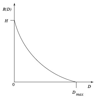
Perceptual distortion is a famous metric that has been used historically for assessing video quality. Distortion theory provides the framework to study the trade-offs between the data rate and the Distortion itself.
In the graph above: Y-axis is the data rate and X-axis the distortion level. If you have a high data rate and a zero distortion, it is a lossless compression scheme.
As soon as cost/spend limitations are considered (in the form of bandwidth and/or storage), data reduction rates will increase and image distortion will appear.
Mean Square Error

Another measure of distortion is mean square error, where is X the input data sequence, Y is output data sequence and N is the count of elements:
Peak-Signal-To-Noise Ratio (PSNR)
Then there is the Peak-Signal-To-Noise ratio (PSNR) which is calculated by comparing the size of an error relative to the peak value of a signal.
The higher the PSNR, the better the video quality. Signal-to-noise ratios are typically expressed in decibel units (dB).
A good ratio will register values of around 80db.
Having explained the metrics used to evaluate the accuracy and quality of lossy compression, it’s time to discuss how the compression process works.
Lossy Compression: the “two” step process
Step 1: Quantization
The step that adds the most distortion is quantization.
Quantization is the process of mapping input from a large set (like an analog signal) to numerical output values in a smaller (usually finite) set.
There are 3 different forms of quantization: uniform, non-uniform, vector.
- Uniform scalar quantizer – subdivides the domain of the input into output values at regular intervals, with the exceptions at the two outer extremes.
- Non-uniform quantizer – output values are not at equally spaced intervals. The output of the reconstructed value that corresponds to each interval is taken during quantization, the midpoint of this interval and the length of each interval is then referred to as the step size which can be denoted by a symbol.
- Vector quantizer – high decoding complexity, output values can be distributed irregularly, not in a grid fashion – such as in the scalar quantizer case – because an output value represents a vector and not a scalar value.
Step 2: Transform coding
Transform coding is the second step in Lossy Compression.
Transform coding is the process of creating a quantized group of blocks (containing all pixels in a frame) of consecutive samples from a source input and converting it into vectors.
The goal of transform coding is to decompose or transform the input signal into something easier to handle.
There is a good chance that there will be substantial correlations among neighboring samples; to put it in other words, adjacent pixels are usually similar, therefore, a compressor will remove some samples to reduce file size.
The range of pixels that can be removed without degrading quality irreparably is calculated by considering the most salient ones in a block.
For example: If Y is the result of a linear transform T of the input vector X in such a way that the components of Y are much less correlated, then Y can be coded more efficiently than X.
If most information is accurately described by the first few components of a transformed vector Y, then the remaining components can be coarsely quantized, or even set to zero, with little signal distortion.
As correlation decreases between blocks and subsequent samples, the efficiency of the data signal encode increases.
Spatial frequency is one of the most important factors of transform coding because it defines how an image (and the pixels within it) change throughout playback in relation to previous and future pixel blocks.
This graphs here depicts two variations:
Spatial frequency indicates how many times pixel values change across an image block. It’s key to note – the human eye is less sensitive to higher spatial frequency components associated with an image than lower spatial frequency components.
If amplitude (learn more about frequency components metrics here) falls below a predefined threshold, it will not be detected by the average human eye.
A signal with high spatial frequency can be quantized more coarsely and therefore maintain quality at lower data rates than a signal with low spatial frequency, which will need more data to provide the user with high perceived quality.
One of the other factors is – Discrete Cosine Transform (DCT) implements the measure of motion by tracking how much image content changes corresponding to the numbers of cycles of the cosine in a block.
The DCT is part of the encoding algorithm and converts pixel values in an image block to frequency values, which can be transmitted with lower amounts of data.
DCT is lossless – apart from rounding errors – and spatial frequency components are called coefficients. The DCT splits the signal into a DC – direct current component and an AC, alternating current component.
With the IDCT or Inverse Discrete Cosine Transform, the original signal is reconstructed and can be decoded and played back.
Step 2.5: Other Transformation Formats
Wavelet
An alternative method of lossy compression is wavelet transformation; which represents a sigma with good resolution in both time & frequency and utilizes a set of functions, called wavelets to transform to decompose an input signal.
Wavelet-coding works by repeatedly taking averages and differences by keeping results from every step of different image parts, this is (almost) a multi-resolution analysis.

A wavelet transform creates progressively smaller summary images from the original, decreasing by a quarter of the size for each step. A great way to visualize wavelet coding is to consider a pyramid – stacking a full-size image, quarter-size image, sixteenth-size image, and so on, on top of each other.
The image has gone through a process of subsampling (through the wavelet transformation algorithm) decreasing the size but aiming at maintaining the quality in smaller iterations.
The image on the right in the top left quadrant has a compressed representation of the full-scale image on the left, which can be reconstructed from the smaller one by applying the wavelet coding transformation inversely.
Another example of lossy compressing a white and black image is:

2D Haar Transform
2D Haar Transform is the representation of a signal with a discrete non-differentiable (step) function – consider a function that represents on/off states of a device.
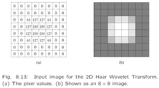
In the context of image decomposition for a simple image applying the 2D Haar Transform would look like:
The image on the left represents the pixel values of the image on the right, an 8 x 8 image.
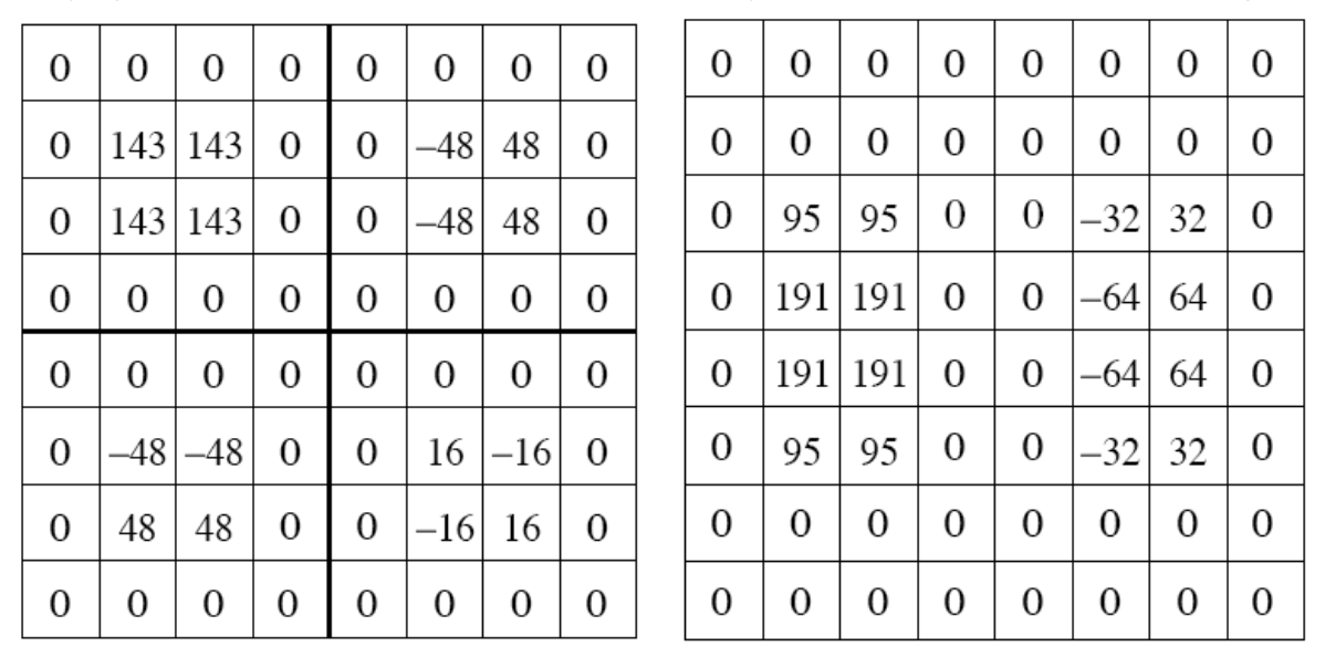
Applying a 2D Haar Transform for the second level, yields a linear decrease of the image size:
The calculated differences and image decrease allow for the image to be compressed with less data while keeping an eye on quality.
More compression means lower quality and higher quality means lower compression.

In the case of color images, the same applies:
In short, the goal of all compression algorithms is to achieve the highest possible compression ratio. For any video distributor compression ratios come to down to cost and quality considerations.
Which trade-off will yield the highest ROI? High compression and high quality at higher costs? The opposite? Or somewhere in the middle?
That’s for you to decide!
Did you enjoy this post? Check out our Video Developer Network for the full university quality videos. (including a lesson on Lossless Compression)
More video technology guides and articles:
- Encoding Definition and Adaptive Bitrate: Video Compression Guide
- Back to Basics: Guide to the HTML5 Video Tag
- What is a VoD Platform? A comprehensive guide to Video on Demand (VOD)
- Video Technology [2022]: Top 5 video technology trends
- HEVC vs VP9: Modern codecs comparison
- What is the AV1 Codec?
Did you know?
Bitmovin has a range of VOD services that can help you deliver content to your customers effectively.
Its variety of features allows you to create content tailored to your specific audience, without the stress of setting everything up yourself. Built-in analytics also help you make technical decisions to deliver the optimal user experience.
Why not try Bitmovin for Free and see what it can do for you.
FAQs
What’s the difference between lossy and lossless compression?
Lossy compression produces an approximation of the original content with some data loss for much higher size reduction. Lossless methods preserve all original information but usually achieve lower compression ratios.
How do developers measure the quality impact of lossy compression?
Developers use distortion metrics like Perceptual Distortion, Mean Square Error (MSE), and Peak Signal-to-Noise Ratio (PSNR) to quantify quality degradation and trade quality vs. bitrate.
Why does lossy compression work well for video but not for text or code?
Because human perception tolerates some inaccuracies in images and audio, lossy methods can discard non-essential information without noticeable quality loss, something unacceptable for exact data like text.
What are common transform techniques used in lossy compression?
Transform coding (e.g., Discrete Cosine Transform, wavelets) converts raw data into components that can be quantized more effectively, concentrating information into fewer bits.

