

TL;DR
- VVC (H.266) is the successor to HEVC (H.265), finalized in 2020 by the Joint Video Experts Team (JVET), targeting significantly improved compression efficiency
- Up to ~50% better compression efficiency than HEVC is achievable at equivalent visual quality, enabling lower bitrates for the same resolution and quality targets
- Designed for next-generation video use cases, including 4K, 8K, HDR, 360° video, AR/VR, and immersive media applications
- Technical advancements include improved block partitioning, motion compensation, and intra/inter prediction tools
- Adoption considerations include computational complexity, encoding performance, and ecosystem readiness, which influence commercial deployment timelines
What is VVC?
Versatile Video Coding (VVC) is the most recent international video coding standard which was finalized in July of 2020. It is the successor to High-Efficiency Video Coding (HEVC) as it was also developed jointly by the ITU-T and ISO/IEC.
So what is really new in VVC? Is this a real revolution when it comes to video coding? In short: No. While it is technically highly advanced, it is only an evolutionary step forward from HEVC. It still uses the block-based hybrid video coding approach, an underlying concept of all major video coding standards since h.261 (from 1988). In this concept, each frame of a video is split into blocks and all blocks are then processed in sequence.
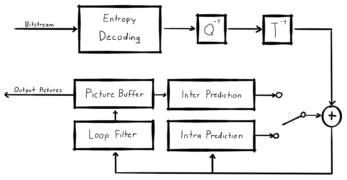
The decoder processes every block in a loop, which starts with entropy decoding of the bitstream. The decoded transform coefficients are then put through an inverse quantization and an inverse transform operation. The output, which is an error signal in the pixel domain, then enters the coding loop and is added to a prediction signal. There are two prediction types. Inter Prediction, which copies blocks from previously coded pictures (motion compensation), and Intra Prediction, which only uses decoded pixel information from the picture being decoded. The output of the addition is the reconstructed block that is put through some filters. This usually includes a filter to remove blocking artifacts that occur at the boundaries of blocks, but also more advanced filters can be used. Finally, the block is saved to a picture buffer so it can be output on a screen once decoding is done and the loop can continue with the next block.
At the encoder side, the situation is a little more complex as the encoder has to perform the corresponding forward operations, as well as the inverse operations from the decoder to obtain identical information for prediction.
Although VVC also uses these basic concepts, all components have been improved and/or modified with new ideas and techniques. In this blog post, I will show some of the improvements that VVC yields. However, this is only a small selection of new tools in VVC as a full list of all details and tools could easily fill a whole book (and someone else probably already started writing one).
VVC Coding structure
Slices Tiles and Subpictures
As mentioned above, each frame in the video is split into a regular grid of blocks. In VVC the size of these so-called Coding Tree Units (CTU) was increased from 64×64 in HEVC to 128×128 pixels. Multiple blocks can be arranged into logical areas. These are defined as Tiles, Slices, and Subpictures. Although these techniques are already known from earlier codecs, the way they are combined is new.

The key feature of these regions is that they are also logically separated in the bitstream and enable various use-cases:
- Since each region is independent, both the encoder and the decoder can implement parallel processing.
- A decoder could choose to only partially decode the regions of the video that it needs. One possible application is the transmission of 360 videos where a user is only able to see parts of a full video.
- A bitstream could be designed to allow the extraction of a cropped part of the video stream on the fly without re-encoding. [JVET-Q2002]
Block Partitioning
Let’s go back to 128×128 CTU blocks. As I mentioned before, the coding loop is traversed for each block. However, processing only full 128×128 pixel blocks would be very inefficient, so each CTU is flexibly split into smaller sub-blocks and the information on how to split it is encoded into the bitstream. The encoder can choose the best division of the CTU based on the content of the block. In a rather uniform area, bigger blocks are more efficient. Whereas in areas with edges or more detail, smaller blocks are typically chosen. The partitioning in VVC is performed using two subsequent hierarchical trees:
- Quaternary tree: There are two options for each block. Do not split the block further or split it into four square sub-blocks of half the width and half the height. For each sub-block, the same decision is made again in a recursive manner. If a block is not split further, the second three is applied.
- Multi-type tree: In the second tree, there are multiple options for each block. It can be split in half using a single vertical or horizontal split. Alternatively, it can be split vertically or horizontally into three parts (ternary split). As for the first tree, this one is also recursive and each subblock can be split using the same four options again. The leaf nodes of this tree that are not split any further are called Coding Units (CUs) and these are processed in the coding loop.
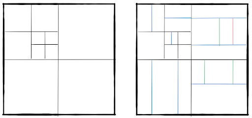
The factor that distinguishes VVC from other video codecs is the high flexibility of block sizes and shapes that a CTU can be split into. With this, an encoder can flexibly adapt to a wide range of video characteristics that result in better coding performance. Of course, this high flexibility comes at a cost. The encoder must consider all possible splitting options which require more computation time. [JVET-Q2002]
Block Prediction
Intra Prediction
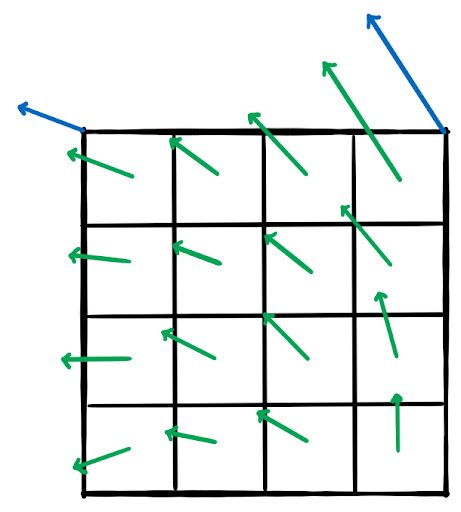
In intra prediction, the current block is predicted from already decoded parts of the current picture. To be more precise, only a one-pixel wide strip from the neighborhood is used for normal intra prediction. There are multiple modes on how to predict a block from these reference pixels. Well-known modes that are also present in VVC are Planar and DC prediction as well as Angular Prediction. While the number of discrete directions for the angle was increased from 33 to 65 in VVC, not much else changed compared to HEVC. So, let’s concentrate on tools that are actually new:
- Wide Angle Intra Prediction: Since prediction blocks in VVC can be non-square, the angels of certain directional predictions are shifted so that more reference pixels can be used for prediction. Effectively this extends the directional prediction angles to values beyond the normal 45° and below -135°. [JVET-P0111]
- Cross-component Prediction: In many cases (e.g. when there is an edge in the block) the luma and chroma components carry very similar information. In cross-component prediction, this is exploited by direct prediction of the chroma components from the reconstructed luma block using a linear combination of the reconstructed pixels with two parameters: a factor and an offset where the factors are calculated from the intra reference pixels. If necessary, scaling of the block is performed as well. [JVET-Q2002]
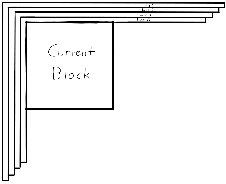
Multi Reference Line Prediction: As mentioned before, only one row of neighboring pixels is used for intra prediction. In VVC, this restriction is relaxed a bit so that prediction can be performed from two lines that are not directly next to the current block. However, there are several restrictions to this as only one line can be used at a time and no prediction across CTU boundaries is allowed. These limitations are necessary for efficient hardware implementations. [JVET-L0283]
Of course, this list is not complete and there are several more intra prediction schemes which further increase the coding efficiency. The method of intra mode prediction and coding of the mode was improved and refined as well.
Inter prediction
For inter prediction, the basic tools from HEVC were carried over and adapted. For example, the basic concepts of uni- and bi-directional motion compensation from one or two reference pictures are mostly unchanged. However, there are some new tools that haven’t been used like this in a video coding standard before:
Bi-directional optical flow (BDOF): If a prediction block uses bi-prediction with one of the references in the temporal past and the second one in the temporal future, BDOF can be used to refine the motion field of the prediction block. For this, the prediction block is split into a grid of 4×4 pixel sub-blocks. For each of these 4×4 blocks, the motion vector is then refined by calculating the optical flow using the two references. While this adds some complexity to the decoder for the optical flow calculation, the refined motion vector field does not need to be transmitted and thus the bitrate is reduced. [JVET-J0024]
Decoder side motion vector refinement: Another method that allows for the motion vectors to automatically be refined at the decoder without the transmission of additional motion data is to perform an actual motion search at the decoder side. While this basic idea has been around for a while, the complexity of a search at the decoder side was always considered too high until now. The process works in three steps:
- First, a normal bi-prediction is performed, and the two prediction signals are weighted into a preliminary prediction block.
- Using this preliminary block, a search around the position of the original block in each reference frame is performed. However, this is not a full search as an encoder would perform it, but a very limited search with a fixed number of positions.
- If a better position is found, the original motion vector is updated accordingly. Lastly, bi-prediction with the updated motion vectors is performed again to obtain the final prediction. [JVET-J1029]
Geometric Partitioning: In the section about block partitioning it was shown how each CTU can be split into smaller blocks. All of these splitting operations only split rectangular blocks into smaller rectangular blocks. Unfortunately, natural video content typically contains more curved edges that can only poorly be approximated using rectangular blocks. In this case, Geometric Partitioning allows the non-horizontal splitting of a block into two parts. For each of the two parts, motion compensation using independent motion vectors is performed and the two prediction signals are merged together using a blending at the edge.
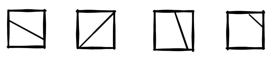
In the current implementation, there are 82 different geometric partition modes. They are made up of 24 slopes and 4 offset values for the partition line. However, the exact number of modes is still under discussion and may still change. [JVET-P0884, JVET-P0085]
Affine motion: Conventional motion compensation using one motion vector can only represent two-dimensional planar motion. This means that any block can be moved on the image plane in x and y directions only. However, in a natural video, strictly planar motion is quite rare and things tend to move more freely (e.g. rotate and scale). VVC implements an affine motion model that uses two or three motion vectors to enable motion with four or six degrees of freedom for a block. In order to keep the implementational complexity low, the reference block is not transformed on a pixel basis, but a trick is applied to reuse existing motion compensation and interpolation methods. The prediction block is split into a grid of 4×4 pixel blocks. From the two (or three) control point motion vectors, one motion vector is calculated for each 4×4 pixel block. Then, conventional two-dimensional planar motion compensation is performed for each of these 4×4 blocks. While this implementation is not a truly affine motion compensation it is a good approximation and allows for very efficient implementation in hard- and software. [JVET-O0070]
Transformation and Quantization
The transformation stage went through some major refactoring as well. Rectangular blocks that were introduced by the ternary split are now supported by the transformation stage by performing the transform for each direction separately. The maximum transform block size was also increased to 64×64 pixels. These bigger transform sizes are particularly useful when it comes to HD and Ultra-HD content. Furthermore, two additional types of transform were added. While the Discrete Cosine Transform in variant 2 (DCT-II) is already well known from HEVC, one further variant of the DCT (the DCT-VIII) was added, as well as one Discrete Sine Transform (DST-VII). Depending on the prediction mode, an encoder can choose different transforms depending on which one works best.
The biggest change to the Quantization stage is the increase in the maximum Quantization Parameter (QP) from 51 to 63. This was necessary as it was discovered that even at the highest possible QP setting, the coding tools of VVC worked so efficiently that it was not possible to reduce the bitrate and quality of certain encodes to the needed levels.
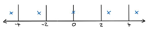
One more really interesting new tool is called Dependent Quantization. The purpose of the quantization stage is to map the output values from the transformation, which are continuous, onto discrete values that can be coded into the bitstream. This operation inherently comes with a loss of information. The coarser the quantization is (the higher the QP value is), the more information is lost. In the figure below, a simple quantization scheme is shown where all values between each pair of lines are quantized to the value of the marked blue cross. Only the index of the blue cross is then encoded into the bitstream and the decoder can reconstruct the corresponding value.
Typically, only one fixed quantization scheme is used in a video codec. In Dependent Quantization, two of these quantization schemes are defined with slightly shifted reconstruction values.
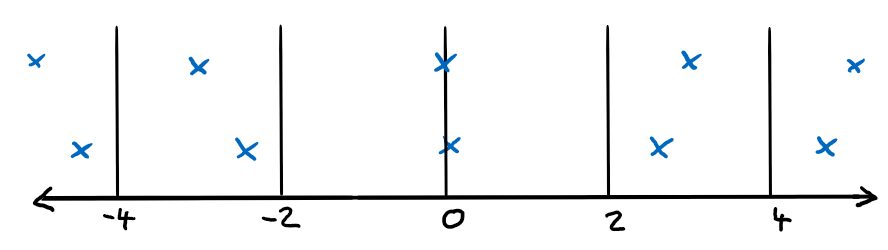
Switching between the two quantizers happens implicitly using a tiny state machine that uses the parity of the already coded coefficients. The encoder can then switch between the quantizers by deliberately changing some of the reconstruction values. Finding the optimal place for this switch where the introduced error is lowest, and the switch gives the most gain can be performed using a rate-distortion trade-off. In some manner, this is related to Sign Data Hiding (used in HEVC) where also information is “hidden” in other data. [JVET-K0070]
Other
All tools discussed so far were built and optimized for the coding of conventional natural two-dimensional video. However, the word `versatile` in its name indicates that VVC is meant for a wide variety of applications. And indeed VVC includes some features for more specific tasks which make it very versatile. Former codecs typically put these specialized tools into separate standards or separate extensions. One such tool is the Horizontal Wrap Around Motion Compensation. A widespread method of transmission of 360° content is to map the 360° video onto a 2D plane using equi-rectangular projection. The 2D video can then be encoded using conventional 2D video coding. However, the video has some special properties which can be used by the encoder. One property is that there is no left or right border in the video. Since the 360° view wraps around, this can be used for motion compensation. So when motion compensation from outside of the left boundary is performed, the prediction wraps around and uses pixel values from the right side of the picture.
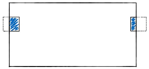
While this tool increases the compression performance it also helps to improve the visual quality since normal video codecs tend to produce a visible edge at the line where the left and right side of the 2D video are stitched back together. [JVET-L0231]
Another application of video coding is the coding of computer-generated video content, also referred to as screen content. This type of content usually has some special characteristics like very sharp edges and very homogeneous areas which are atypical for natural video content. One very powerful tool in this situation is Intra Block Copy which performs a copy operation from the already decoded area of the same frame. This is very similar to motion compensation with the key difference that the signalled vector does not refer to a temporal motion but just points to the source area in the current frame for the copy operation. [JVET-J0042]
Coding performance
With every Standardization meeting, the VVC test model software (VTM) is updated and a test is run to compare the latest version of VTM to the HEVC reference software (HM). This test is purely objective using PSNR values and the Bjøntegaard delta. While multiple different configurations are tested, we will focus on the so-called Random-Access configuration which is the most relevant when it comes to video transmission and streaming. 
BD-rate comparison of VTM 7.0 compared to HM 16.20. [Q0003]
In terms of BD-rate performance, VTM is able to achieve similar PSNR values while reducing the required bandwidth by roughly 35%. While the encoding time is not a perfect measure of complexity it can give a good first indication. The complexity of VVC at the encoder side is roughly 10 times higher, while the decoder complexity only increases by a factor of 1.7. Please note that these results are all based on PSNR results. It is well known that PSNR values are not that well coupled to the actual subjectively perceived quality and some preliminary experiments show that the subjective results seem to be higher than 35% bitrate reduction. A formal subjective test is planned for later this year.
Conclusion
So after all of this technical detail what is the future of VVC going to be? From a technical side, VVC is the most efficient and advanced coding standard that money can buy. However, it is unknown as of yet how much it will really cost. Once the standardization process is officially finished in October 2020, the process to establish licensing terms for the new standard can be started. From previous standards, we have learned that this is a complicated process that can take a while. At the same time, there are other highly efficient codecs out there for which applications and implementations are maturing and evolving.
Links and more information
The JVET standardization activity is a very open and transparent one. All input documents to the standardization are publicly available here. Also, the reference encoder and decoder software are publicly available here.
Bitmovin & Standardization
Bitmovin is heavily involved in the standardization process around back-end vidtech; this includes our attendance and participation in the quarterly MPEG meetings, as well our membership and involvement in AOMedia.
Video technology guides and articles
- Back to Basics: Guide to the HTML5 Video Tag
- What is a VoD Platform?A comprehensive guide to Video on Demand (VOD)
- Video Technology [2022]: Top 5 video technology trends
- HEVC vs VP9: Modern codecs comparison
- What is the AV1 Codec?
- Video Compression: Encoding Definition and Adaptive Bitrate
- What is adaptive bitrate streaming
- MP4 vs MKV: Battle of the Video Formats
- AVOD vs SVOD; the “fall” of SVOD and Rise of AVOD & TVOD (Video Tech Trends)
- MPEG-DASH (Dynamic Adaptive Streaming over HTTP)
- Container Formats: The 4 most common container formats and why they matter to you.
- Quality of Experience (QoE) in Video Technology [2022 Guide]
FAQs
What is VVC (H.266)?
VVC (Versatile Video Coding), also known as H.266, is a video compression standard developed to succeed HEVC. It was finalized in 2020 and is designed to reduce bitrate requirements by roughly 50% compared to HEVC while maintaining the same perceptual quality.
How does VVC achieve better compression than HEVC?
VVC introduces more flexible block partitioning structures, enhanced motion vector prediction, advanced intra and inter prediction techniques, and improved transform and entropy coding mechanisms. These innovations collectively increase coding efficiency across a wide range of resolutions and content types.
Is VVC better than HEVC?
From a compression efficiency standpoint, yes. VVC can deliver equivalent visual quality at significantly lower bitrates. However, trade-offs include higher encoding complexity and ecosystem maturity considerations.
What use cases is VVC designed for?
VVC is optimized for high-resolution and next-generation formats, including:
– 4K and 8K streaming
– High Dynamic Range (HDR)
– 360° and immersive video
– Augmented and virtual reality experiences
1. What is VVC (H.266)?
VVC (Versatile Video Coding), also known as H.266, is a video compression standard developed to succeed HEVC. It was finalized in 2020 and is designed to reduce bitrate requirements by roughly 50% compared to HEVC while maintaining the same perceptual quality.
2. How does VVC achieve better compression than HEVC?
VVC introduces more flexible block partitioning structures, enhanced motion vector prediction, advanced intra and inter prediction techniques, and improved transform and entropy coding mechanisms. These innovations collectively increase coding efficiency across a wide range of resolutions and content types.
3. Is VVC better than HEVC?
From a compression efficiency standpoint, yes. VVC can deliver equivalent visual quality at significantly lower bitrates. However, trade-offs include higher encoding complexity and ecosystem maturity considerations.
4. What use cases is VVC designed for?
VVC is optimized for high-resolution and next-generation formats, including:
– 4K and 8K streaming
– High Dynamic Range (HDR)
– 360° and immersive video
– Augmented and virtual reality experiences