Everyone knows what a jpeg is! It’s an image of course.
Yes and No – JPEG is the acronym that sits at the end of your picture file on your favorite device. You must be thinking, “Hold on one second, if it’s not the actual image, and it’s an acronym, what is it and what does it stand for?” Keep reading to find out:
Do I look like I know what a JPEG is?

You may know the meme, do you actually know? JPEG is one of the world’s most common lossy image compression standards and stands for Joint Photographic Experts Group. JPEG is defined as a working group within the International Organization for Standardization (ISO/IEC). It’s important to note that JPG and JPEG are the same, however, the former was used in Windows because file name extensions could only have three letters.
The process of compressing an image in a lossy way is to convert it from the raw format to JPEG, whereby the image is split into blocks (ex: 8×8 pixels), separated, and organized using the Discrete Cosine Transform (learn more about DCT). The image is described as a function in the spatial domain in this step of the data compression process. The effectiveness of JPEG when using DCT as a transfer encoding (effectively mapping input values to output values, using less data) is based on three major observations: saliency in an image, spatial redundancy, and visual acuity.
Deciding if it “Needs More JPEG”
To measure the effectiveness and quality of lossy compression, you need to understand these observations in detail:
Image Saliency
The focal point (or salience) of an image changes slowly across an image. it is unusual for pixel intensity values to vary multiple times in a small area, for example within an 8×8 image block. The majority of data in a pixel block is repeated, this is known as “spatial redundancy.” The same applies to the rest of the blocks in an image. That’s why it’s possible to represent an image with less data than the original content without sacrificing quality.
Spatial Redundancy
Psychophysical experiments suggest that people are much less likely to notice the loss of very high spatial frequency components than the loss of lower frequency components. For example, high-frequency components can be white pixels in consecutive image blocks on a white background, whereas low-frequency components like facial features in close up scenes are much more noticeable. Thus, high spatial frequency components are exploited by applying the DCT on them to considerably decrease the spatial redundancy in an image (and therefore in a video). The outcome of this process is a lower expenditure on bits when transmitting an image of similar quality as the original.
Visual Acuity
Visual Acuity is the measurement of a viewer’s ability to accurately distinguish closely spaced lines. For example, the difference between gray variants (black & white scale) can be distinguished with much greater accuracy and ease than color variants. Other than RGB, color in an image can be represented with three channels: one for luminance and two for chroma samples, YCbCr. This concept is applied in JPEG in the context of Chroma subsampling; which utilizes visual acuity to use more information when encoding brightness (luminance), as the human eye has a higher sensitivity towards luminance than for color differences (chrominance). The most common specification for chroma subsampling is a 4:2:2 ratio – as defined below:
Y:Cb:Cr – Y is the width in pixels of the sampling reference, Cb is the number of chroma values, and Cr is the number of changes in the chroma values.
In a 4:2:2 ratio, luminance has twice the sample rate of the chrominance. When the ratio is 4:4:4 – there is no chroma subsampling. The combined assumptions that image information varies relatively slowly, people are less likely to notice the loss of highly frequent components, and that luminance takes visual priority in human sight are the theoretical frameworks behind implementing a JPEG encoder.
Encoding images – processes defined
A full JPEG encoding process is best visualized using the following block diagram:
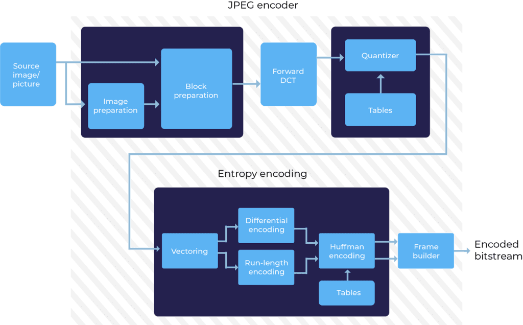
The process begins with a source image that’s prepared for encoding using chroma subsampling.
Discrete Cosine Transform
After the chroma subsample ratios are set, the image is split into 8×8 blocks:
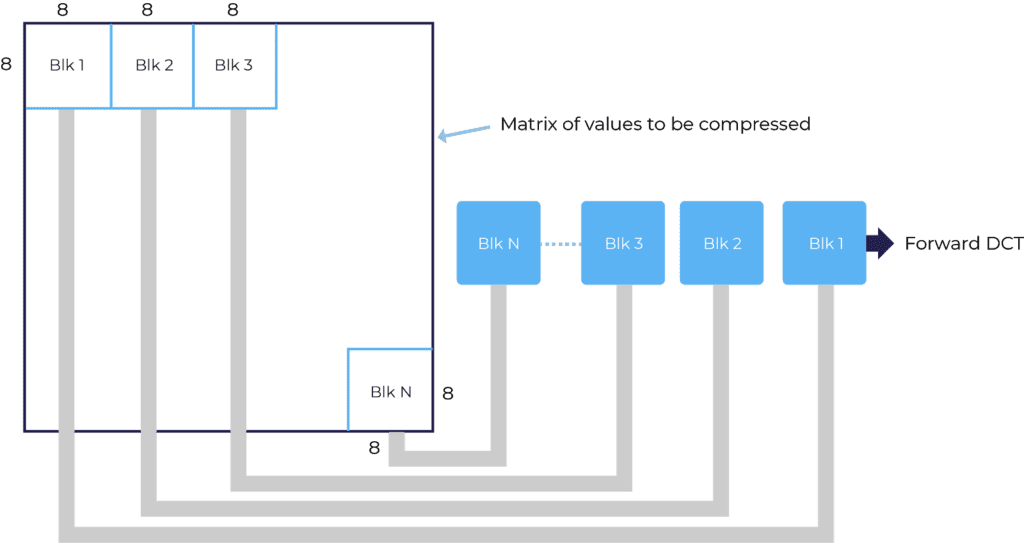
Using a block diagram, each block is processed independently of the others. Forward DC is then applied individually to each of these blocks, successive image block analysis (backward DCT analyzes previous blocks). An image must be split into blocks and individually transformed, otherwise, applying high compression ratios will result in a blocky JPEG image. An encoder will vector an image using a Zig-Zag scanning method (from the top left-hand corner to bottom right-hand corner). The graphic below illustrates this process:
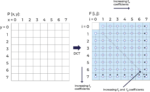
Applying DCT will split the image from the upper left to the lower right corner into AC and DC coefficients. DCT coefficients are further divided into corresponding values of a quantization matrix. As illustrated below:
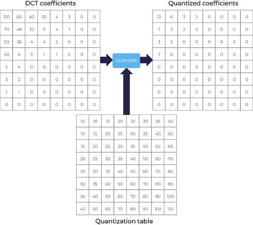
Quantization
Applying quantization rounds up various integers, therefore introducing loss into the compression process. Higher frequency components have higher quantization table integer values. JPEG has predefined quantization tables for luminance and for chrominance components. Regardless of the content type (image, audio, or video), the goal of an encoder is to maximize the compression ratio and minimize the perceptual loss in transferred content.
By separating frequency components, lower frequency components that map to 0 in the quantization table can be filtered out; therefore increasing the compression capacity. More 0s = more compression!
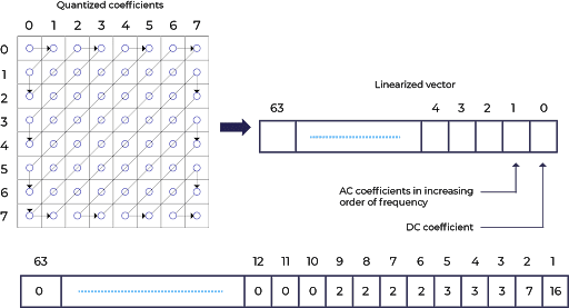
Next, the image is split into even smaller blocks, any variations across these blocks are measured over time. The next step after quantization is taking the Qantas coefficients (values extracted during quantization) and creating a vector with quantized values.
Coding Coefficients
Successively, the encoder will perform a Run-length Coding (RLC) algorithm on the AC Coefficients. Run-length coding replaces frequency values with a pair of integers: the run-length value, which specifies the number of zeros in the run and the value of the next non-zero AC coefficient. Unlike AC, DC components use Differential coding after vectoring, where the first value of the DC coefficient is coded as is and the remaining values are coded as “different”. This process is illustrated below:
Once the RLC and differential codes are complete, both AC and DC coefficients undergo entropy coding. Entropy coding defines AC and DC values by size and amplitude; where size indicates the count of used and amplitude is the value of the bits.
The final coding step that the AC and DC components will pass through is the Huffman coding algorithm. Only “size” is Huffman coded as smaller sizes occur more often in an image. Amplitude is not, as its value can change so widely that Huffman coding will have no appreciable benefit. This method is applied for every block the image has been split up into.
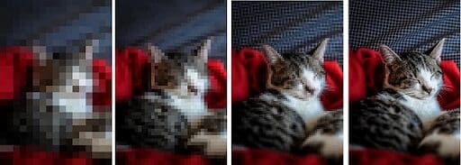
Bitstreams
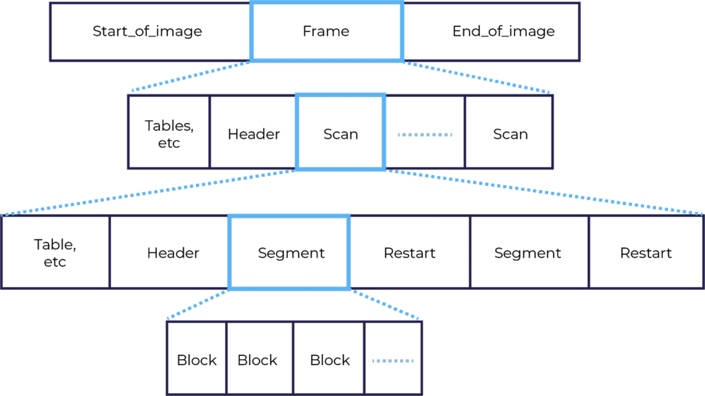
The resulting output needs to be put in a bitstream, also known as a binary sequence. There are many modes of bitstreams, JPEG uses a progressive mode. Which quickly delivers a low-quality version of the image, followed by higher quality passes. The JPEG bitstream is illustrated below:
Using a progressive mode, the most significant bits are downloaded first, followed by less significant ones. The result is an image that increases in quality as more blocks are progressively decoded from the Most Significant Bit (MSB) to the Least Significant Bit (LSB). This means that your browser is effectively doing multiple decodes as more information added over time. An example of progressive JPEG decoding over time:
Did you enjoy this post and do you want to learn more about compression algorithms?
This post is a part of our Video Developer Network, the home of free university-level courses about back-end video technology. Check the links below for relevant content:
[Landing Page] Video Developer Network
[Developer Network Lesson] Image Compression Standards
[Blog] Developer Network Series: Everything you need to know about Lossy Compression Algorithms